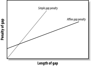
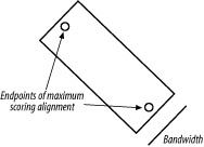
3.6 Variations

The algorithms as described and implemented earlier are rarely used. Over the years, important innovations have made the general algorithms more applicable to aligning biological sequences and running efficiently in a computer.

3.6.1 Gap Modifications

Most alignment algorithms employ affine gaps. The previous description used a simple gap-scoring scheme in which every letter inserted or deleted cost the same amount. This isn't a very good model of biology because large gaps tend to occur fairly often. To better model this phenomenon, affine gaps are used where there is a greater penalty for opening a gap than extending the gap. Figure 3-7 shows a graphical view.

Figure 3-7. Comparison of simple and affine gap scoring schemes

Affine gap penalties are a simple modification to either algorithm. All you need to do is to record a third value in each cell of the matrix that keeps track of whether a gap has already been opened or not and then assign the appropriate gap penalty. Some algorithms even allow multiple gap scoring schemes so that very long gaps are not penalized as much. You can visualize how this works by following the minimal penalty in Figure 3-7. These algorithms are slightly more complicated because scores for each affine gap must be tracked. Usually two affine penalties are employed, and the algorithms are labeled double affine.

3.6.2 Reduced Memory

You shouldn't attempt to align long sequences (e.g., genomic DNA) with the versions of Needleman-Wunsch and Smith-Waterman described in Examples Example 3-1 and Example 3-2. The number of cells in the alignment matrix is the product of the sequence lengths, and each cell may take 8 bytes or more of memory. Therefore, aligning two 100,000-bp DNA sequences requires approximately 80 gigabytes (GB) of RAM. Fortunately, there are linear-memory versions of the algorithms.

You may have noticed during the fill phase of the algorithms that you use only two rows at a time. The other rows just sit there, either waiting to be calculated or waiting for the trace-back. Why not just use two rows at a time and not allocate the whole matrix? If you do this, you can calculate the score of the maximum scoring alignment and record its ending coordinates. By reversing direction, you can then compute the starting coordinates. Unfortunately, you lose the ability to perform a trace-back. But the memory required is now just two times the length of one of the sequences rather than the product of the two sequences. Using this approach, you can compare two 100,000-bp DNA sequences in just 1.6 megabytes (MB) of RAM. The alignment algorithm is now O(n) in memory, but still O(nm) in time.

How do you get the actual alignment? Given the coordinates of the maximum scoring alignment you can restrict the search space to a region between the two endpoints (Figure 3-8). With this approach, a diagonal line is drawn between the endpoints, and the search space is restricted to a certain number of cells on either side of the diagonal. The width of the search space is called the bandwidth. If the bandwidth is too small, the alignment will walk along the edge of the band and may no longer follow the path of the maximum score. If the bandwidth is needlessly large, both memory and computation are wasted. Now that the search space is sufficiently small, you can perform a complete fill and trace-back. However, if the alignment is especially large, even this restricted space can be quite large. For this reason, it is common to use a divide-and-conquer strategy that requires twice the computation, but very little memory.

Figure 3-8. Banded alignment

In Example 3-2, most of the cells had a score of zero. Doesn't it seem a waste of time and memory to explore regions in which the score is poor? Why not make alignments only where positive scores are likely? That's exactly the thinking behind BLAST, as discussed in Chapter 5.

3.6.3 Aligning Transcripts to Genomic Sequence

Determining the correct exon-intron structure of genes isn't always easy. One very successful approach is to align transcripts back to their origin in a genome. However, this isn't as simple as it may appear. Several solutions to this problem use either global or local techniques.

A global alignment between a transcript and a genomic sequence is expected to have huge gaps corresponding to the introns. In eukaryotic genomes, such as the human genome, exons may account for only 1 to 2 percent of a genome. As a result, the gap scores may completely dominate the scoring function, and the alignment may be of little consequence. If the gap costs are too low, the alignment may spread out, and exons may not be faithfully aligned. These problems are largely solved by gapping with double affine penalties, but there are still potential problems with short exons and introns.

A standard local alignment between a transcript and a genome typically identifies the longest exon as the maximum scoring pair. This isn't as useful, but many local alignment algorithms, like BLAST, produce more than one alignment. With these variants, mapping a transcript back to a genome is simply a matter of chaining the individual alignments together. This turns out to be another tricky problem, but it works well most of the time